| Prev | Next |
StateMachine Solver Examples
This topic provides some simple examples of where and how to apply Solvers in StateMachine Simulations, which includes using scripts in StateMachine operations as well as in Transition connectors. The images in this topic show Octave Solver examples; however, unless otherwise stated, the same script can be used for MATLAB in the MATLAB Solver.
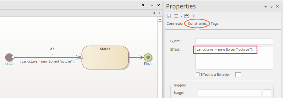
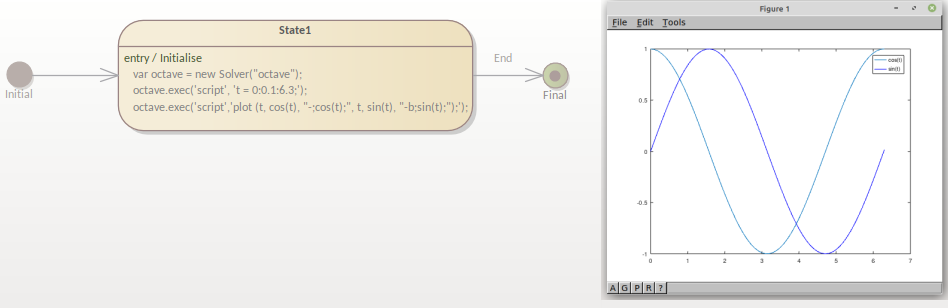
Initializing the Solver
The script to initialize a Solver in a StateMachine can be placed either in the Effect of a Transition or in the Entry operation of a State. It is usually placed in the Effect of the first Transition exiting the Initial.
Assigning Values and Executing Commands
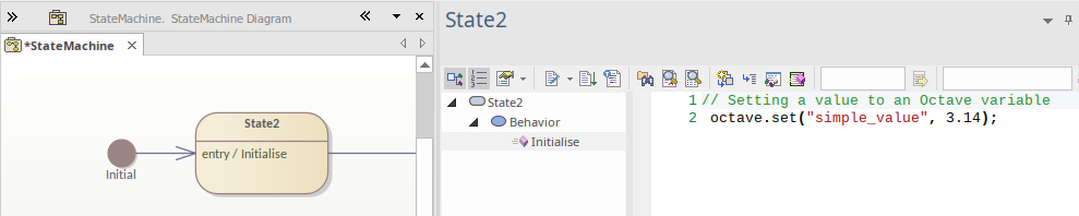
To assign a value, use the octave.set() or matlab.set() function.
For StateMachines the method can be placed in the Effect of a Transition or in the Behavior (Entry/Do/Exit) of an operation.
To edit the Effect of a Transition you use the 'Constraints' page of the 'Properties' dialog.
To place the method in an operation, open the operation's Behavior script:
- Create a new Entry operation in the State from either the diagram or the Browser window, by right-clicking on the element and selecting the 'Features > Operations' context menu option.
- Click on the new Entry operation and press .
This will open the behavior script in the editor.
When executing MATLAB or Octave commands using the .exec() function, the commands can be placed in the Effect of the Transition or the Behavior script of the operation.
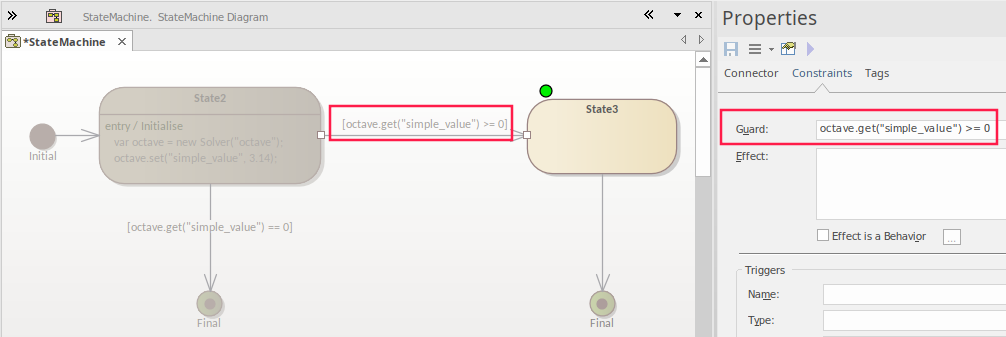
Conditional Branching
When using conditional branching in a StateMachine, the condition can be placed in the Guard of a Transition and can contain a script calling MATLAB or Octave functions. For example:
Note:
- The condition can also be set using a Choice; the placement of the condition statement is the same, in that it is defined in the Guard of the exiting Transition
- The example shows a simulation at the Breakpoint set on State3
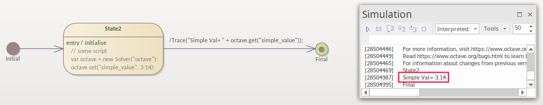
Getting Results
When returning the results from external function calls, you can use the Solver's get() function to return the results in the script. There are three key options for then delivering the results from the script to the user:
- Trace()
- Plot
- Win32 display
With both the Trace and Win32 options you must return a local copy in your JavaScript, using the Solver's .get() command. As an example of using the .get() command, see the Guard in the previous image.
Using Trace
The Trace() command is useful when initially writing and debugging a simulation, as it allows you to check the results of your script at different stages. The results are output in the Simulation window.
Executing Plots
Octave and MATLAB have a strong emphasis on the ability to generate a plot, as this is a key method of outputting results. To generate a plot you use the Solver's .exec() function to call a plot generation function.
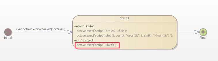
Holding the Plot
When executing a plot in a simulation, if the simulation is not paused the plot will only be viewable for a brief moment. So, for StateMachines, there are two options for pausing the flow while the plot is being viewed:
- Using the uiwait in Octave or MATLAB. For example this can be set in the Exit Operation or an in a Transition Effect. Here is an example using Octave:
octave.exec('script','uiwait');
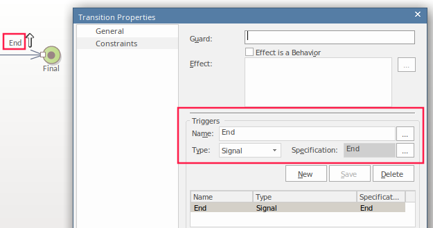
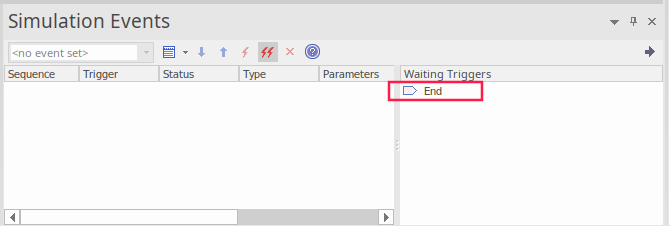
- Setting a Trigger/Event sequence to pause the simulation in a Transition out of the State where the plot was generated. In the example case this is in the final Transition.
To progress past the Transition you can either:
- Click on the Trigger showing in the Simulation Events window or
- Use a BroadcastSignal() from, say, a button in the Win32 screen (this is discussed in the Using the Win32 Interface section, next)
Using the Win32 Interface
When using the Win32 interface the broad steps to perform are:
- Create a Win32 dialog
- Set a script line to open the dialog
- Get a value from a field in the dialog
- Pass that value to the solver
- Use a button to trigger the plot
The steps to configure a Win32 interface are:
- Create a ‘Starter Win32 Model’ using the Start Page 'Create from Pattern' tab (Model Wizard) - select the 'UX Design' Perspective Set and the 'Win32 UI Models' Perspective
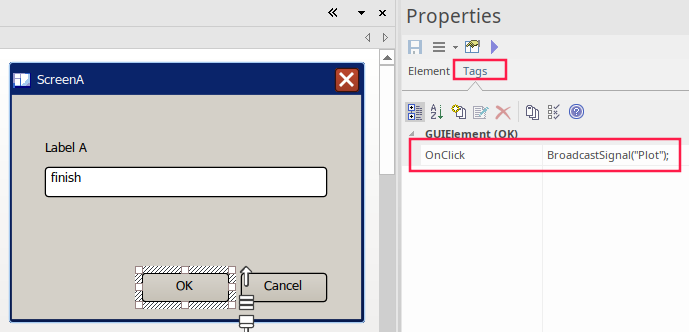
- Change the name of the <<Win32 Screen Dialog>> to 'ScreenA'
- Change the name of ‘Edit Control A’ to something more meaningful, such as ‘finish’
- Click on State1 and press to add - in the Entry Operation's script - a call to open the dialog:
dialog.ScreenA.Show=true;
To get a valid user input value, the user must click on the , so from the OK button you must Broadcast an event for a Trigger to start the process. To receive the Trigger you must have a Signal and set a Transition to be triggered by that Broadcast to the Signal.
See the steps to create and set the Trigger and Signal 'End', as shown in the Using a Trigger to Hold the Plot section, earlier. In this case we are setting the same Transition, but for a new Trigger called 'Plot'. This is sending a BroadcastSignal(‘Plot’) using the OnClick Tagged Value on a button:
The Transition exiting State1 is set to be triggered by the BroadcastSignal:
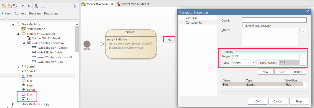
On the Transition you must create a Trigger, set the Trigger-Type to Signal and create the Signal. For more detail see the Win32 User Interface Simulation Help topic.
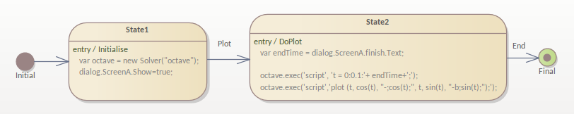
The script to run the plot will be in the Entry operation of State2. During the simulation the transition into State2 will only occur after the Win32 OK button is clicked and the Plot trigger is sent. So we now:
- Add an Entry Operation and open the Behavior using Alt+7
- In this state's Entry Operation we get the value of the field using:
var endTime = dialog.ScreenA.finish.Text;
This sets a variable with the value for the last parameter to be sent to Octave for the plot - In the octave.exec() statement, we place the variable to set the number of seconds to plot too:
octave.exec('script', 't = 0:0.1:'+ endTime+';');
This gives two States with the scripts in the Entry Operations:
Running the Simulation
To run the simulation:
- Select the Simulate ribbon and click on 'Run Simulation > Start'
When you enter a value and click on the , this returns:
